Overview of topics in experimental design
Part 1 — Plackett-Burman Screening
What is it, in plain language?
Imagine you're trying to bake the perfect cake, and you suspect that seven things might affect how good it turns out: oven temperature, baking time, amount of sugar, type of flour, mixing speed, amount of butter, and egg quantity. You want to figure out which of these actually matter the most — but running experiments for every possible combination would take forever (with 7 factors at 2 levels each, that's 2⁷ = 128 experiments!).
Plackett-Burman design is a clever shortcut. It lets you screen many factors using surprisingly few experiments to figure out which ones are important. You won't get a perfect picture of how all the factors interact — but you'll quickly identify the "big hitters" worth investigating further.
Key facts:
- It's a screening design — used early in experimentation to filter many factors down to a few important ones.
- Each factor is tested at just two levels: a "low" value (written as
-or-1) and a "high" value (written as+or+1). - The number of experiments (called "runs") must be a multiple of 4: 8, 12, 16, 20, 24, etc.
- With N runs, you can study up to N − 1 factors.
The Steps
Step 1: List your factors and pick two levels for each
Pick the things you want to test. For each one, choose a sensible "low" and "high" value. The levels should be far enough apart to actually produce a difference, but still realistic.
Step 2: Decide how many runs you need
Use the smallest multiple of 4 that is at least one more than your number of factors.
- 1–3 factors → 4 runs
- 4–7 factors → 8 runs
- 8–11 factors → 12 runs
- 12–15 factors → 16 runs
Step 3: Build the design matrix
A design matrix is a table that tells you exactly what settings to use in each experiment. You build it from a special starting row called a generator row (pre-tabulated in any DOE reference). Then you "shift" the row to make all the other rows, and finish with a row of all -'s.
Step 4: Randomize the run order
Don't run the experiments in the order they appear in the table — shuffle them. This protects you from time-related effects (equipment warming up, weather changing).
Step 5: Run the experiments and record the response
The "response" is whatever you're measuring — yield, strength, taste score, error rate.
Step 6: Calculate the effect of each factor
Effect = (Average response when factor is at +) − (Average response when factor is at −)
A large positive effect means raising that factor increases the response. Close to zero means the factor probably doesn't matter.
Step 7: Identify the important factors
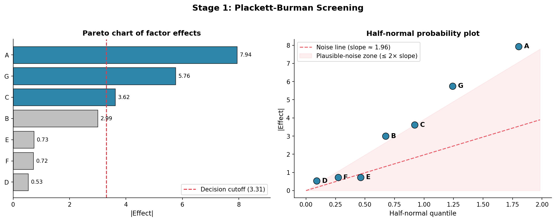
The factors with the largest absolute effects are your "vital few." Plot them on a Pareto chart or half-normal plot to visually separate signal from noise.
A Fully Worked Example
The scenario: You're a chemist trying to maximize the yield (%) of a chemical reaction. You suspect 7 factors could influence yield.
Step 1 — Factors and levels
| Factor | Symbol | Low (−) | High (+) |
|---|---|---|---|
| Temperature | A | 60 °C | 80 °C |
| Pressure | B | 1 atm | 2 atm |
| Catalyst type | C | Type 1 | Type 2 |
| Reaction time | D | 1 hour | 2 hours |
| Mixing speed | E | 100 rpm | 300 rpm |
| pH | F | 6 | 8 |
| Concentration | G | 0.1 M | 0.5 M |
Step 2 — Number of runs
We have 7 factors, so we need at least 8 runs.
Step 3 — Build the design matrix
For an 8-run design, the generator row is + + + − + − −. Write it as Row 1, then cyclically shift (move the last element to the front) to get Rows 2–7. Row 8 is all minuses.
| Run | A | B | C | D | E | F | G |
|---|---|---|---|---|---|---|---|
| 1 | + | + | + | − | + | − | − |
| 2 | − | + | + | + | − | + | − |
| 3 | − | − | + | + | + | − | + |
| 4 | + | − | − | + | + | + | − |
| 5 | − | + | − | − | + | + | + |
| 6 | + | − | + | − | − | + | + |
| 7 | + | + | − | + | − | − | + |
| 8 | − | − | − | − | − | − | − |
Each column has exactly four +'s and four −'s — the balance that makes the math work.
Steps 4–5 — Randomize and run
| Run | A | B | C | D | E | F | G | Yield (%) |
|---|---|---|---|---|---|---|---|---|
| 1 | + | + | + | − | + | − | − | 78 |
| 2 | − | + | + | + | − | + | − | 65 |
| 3 | − | − | + | + | + | − | + | 70 |
| 4 | + | − | − | + | + | + | − | 72 |
| 5 | − | + | − | − | + | + | + | 68 |
| 6 | + | − | + | − | − | + | + | 80 |
| 7 | + | + | − | + | − | − | + | 75 |
| 8 | − | − | − | − | − | − | − | 55 |
Step 6 — Calculate the effects
Factor A (Temperature): + runs 1,4,6,7 → avg 76.25 | − runs 2,3,5,8 → avg 64.50 → Effect = +11.75
Factor B (Pressure): + avg 71.50, − avg 69.25 → Effect = +2.25
Factor C (Catalyst): + avg 73.25, − avg 67.50 → Effect = +5.75
Factor D (Time): + avg 70.50, − avg 70.25 → Effect = +0.25
Factor E (Mixing speed): + avg 72.00, − avg 68.75 → Effect = +3.25
Factor F (pH): + avg 71.25, − avg 69.50 → Effect = +1.75
Factor G (Concentration): + avg 73.25, − avg 67.50 → Effect = +5.75
Step 7 — Rank and interpret
| Factor | Effect |
|---|---|
| A — Temperature | +11.75 |
| C — Catalyst | +5.75 |
| G — Concentration | +5.75 |
| E — Mixing speed | +3.25 |
| B — Pressure | +2.25 |
| F — pH | +1.75 |
| D — Time | +0.25 |
Temperature is the runaway winner. Catalyst type and Concentration are secondary. Mixing, Pressure, pH, and Time show small effects — set them to whichever level is cheapest.
The Pareto chart below visualises this: factors A, G, and C clear the decision cutoff (dashed line), while the rest fall in the noise zone on the half-normal plot.
Part 2 — Full Factorial Design
Once screening identifies the vital few (here: A, C, G), a full factorial design tests every possible combination of those factors. No shortcuts — you cover the entire space.
How it's built
With 3 factors at 2 levels each you run 2³ = 8 experiments:
| Run | A | C | G |
|---|---|---|---|
| 1 | − | − | − |
| 2 | + | − | − |
| 3 | − | + | − |
| 4 | + | + | − |
| 5 | − | − | + |
| 6 | + | − | + |
| 7 | − | + | + |
| 8 | + | + | + |
Every column is balanced, and every pair of columns shows all four combinations equally — that's what lets you estimate interactions cleanly.
Why use it
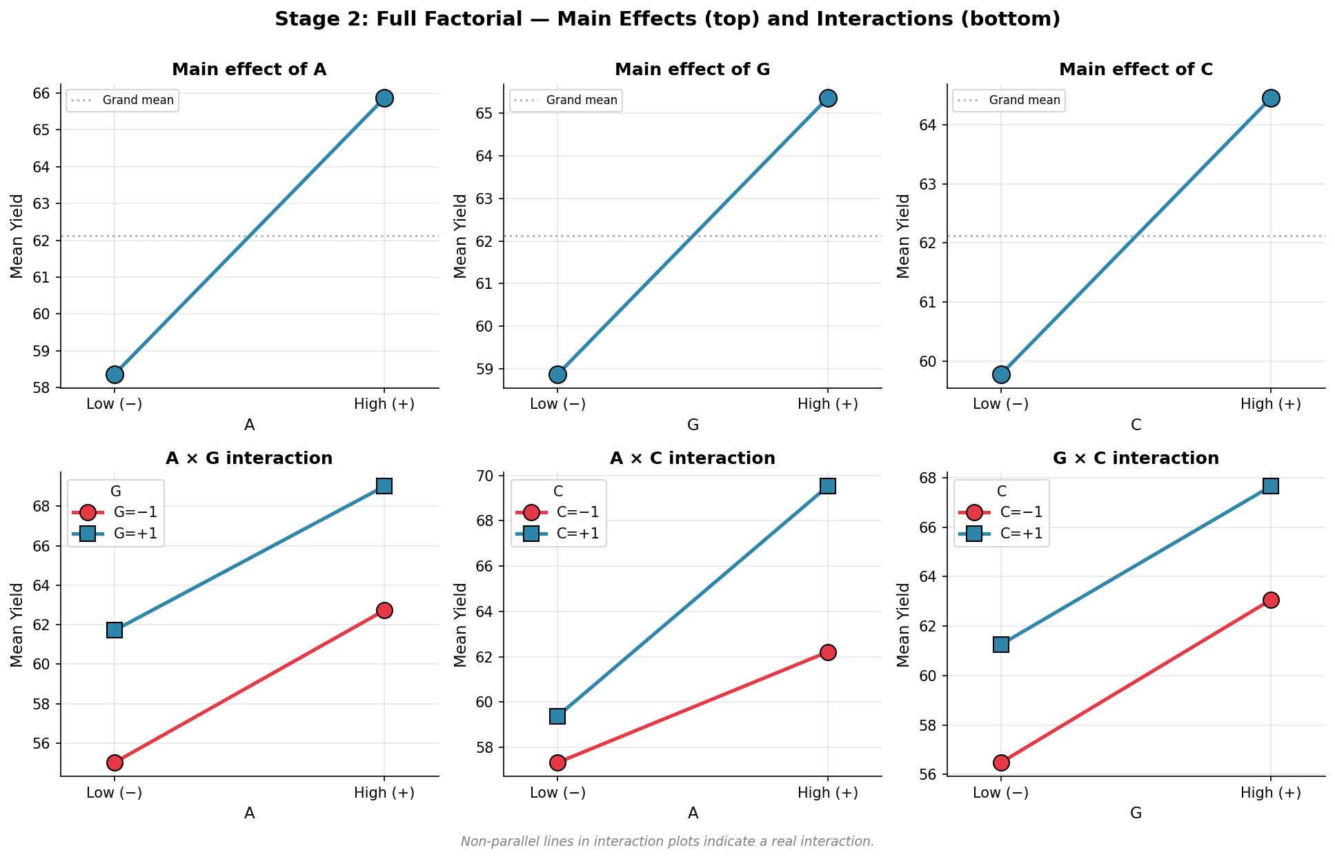
The big payoff over Plackett-Burman is detecting interactions — when the effect of one factor depends on the level of another. "Raising temperature only helps when the catalyst is Type 2" is an interaction; PB is blind to it, a full factorial sees it clearly.
You compute main effects the same way as before. Interaction effects use a derived column: the A×C column is just A × C row by row, and you average the response at + rows minus the − rows.
What you can model
A 2-level full factorial gives you a linear model with interactions:
Yield = β₀ + β₁·A + β₂·C + β₃·G + β₁₂·AC + β₁₃·AG + β₂₃·CG + β₁₂₃·ACG
There are no squared terms — you can't see curvature with only two levels per factor.
The catch
Runs explode fast. 3 factors = 8 runs (fine). 5 factors = 32 runs (painful). 7 factors = 128 runs (impractical). Screen first, then run a full factorial only on the 2–4 survivors.
The plots below show main effects (top row) and interaction plots (bottom row) for factors A, C, G. Non-parallel lines in the interaction plots are the signature of a real interaction — notice A × C: the two lines cross, confirming these two factors interact strongly.
Part 3 — Response Surface Design
A full factorial at 2 levels tells you the direction of each factor but not the shape. A response surface design adds a third level (and sometimes more), so you can map out curves, peaks, and valleys.
Why you need curvature
Imagine yield as a function of temperature. From a 2-level experiment you might see yield going up and conclude "hotter is better." But the true relationship might be a hill — yield rises, peaks at 75 °C, then falls. With data only at 60 °C and 90 °C you'd miss the peak entirely. A third measurement (75 °C) reveals the curve.
Common designs
Central Composite Design (CCD). Start with a 2-level factorial (corners of a cube). Add a center point — a run with every factor at its midpoint. Then add axial points that push one factor past its high/low while the others stay at the center. For 2 factors the geometry looks like a square with a star superimposed: 4 corners + 1 center + 4 star points = 9 runs. The star points are what detect curvature along each axis.
Box-Behnken Design. Skips the corner and extreme axial runs. More efficient when you have many factors and running every factor at its extreme simultaneously would be dangerous or expensive.
What you can model
The fitted model is a full quadratic — squared terms that capture curvature:
Yield = β₀ + β₁·A + β₂·C + β₃·G + β₁₁·A² + β₂₂·C² + β₃₃·G² + β₁₂·AC + β₁₃·AG + β₂₃·CG
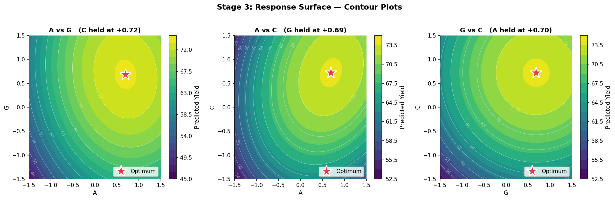
Once you have this equation you can take derivatives, set them to zero, and solve for the optimum. You can also draw contour plots — topographic maps of the response — that show exactly where the peak is and how steep the surrounding slopes are.
The contour plots below show the predicted yield surface for each pair of factors (third factor held at its optimum). The red star marks the predicted optimum.
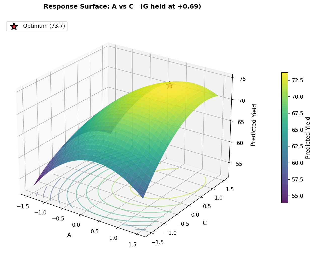
The 3D surface below shows the same A vs C slice: a clear hill with a peak around yield = 73.7, confirming the model has captured the curvature well.
How the Three Stages Fit Together
| Stage | Design | Question answered |
|---|---|---|
| 1. Screening | Plackett-Burman | Of my 7+ factors, which 2–4 actually matter? |
| 2. Characterization | Full factorial (2-level) | How do those factors and their interactions affect the response? |
| 3. Optimization | Response surface (CCD or Box-Behnken) | Exactly what settings maximize the response? |
Each stage uses the results of the previous to focus effort. You start with a wide net and many factors, then progressively zoom in — fewer factors, more levels, more detail.
To close with the cake-baking example: Plackett-Burman might tell you that temperature, time, and sugar are the only factors that really matter. A 2³ full factorial tells you whether temperature and time interact (they almost certainly do). Finally, a response surface design pinpoints the exact combination that produces the perfect cake — including the curvature that says "175 °C is the sweet spot, and going either above or below makes things worse."
Python Simulation
All three stages above are simulated end-to-end in a companion Python project. The script runs the full pipeline — PB screening, full factorial, and CCD response surface — against a known true model so you can see exactly how well each stage recovers reality.
The true underlying process (unknown to the experimenter, known to us) is:
Yield = 70 + 4·A + 0.1·B + 2·C + 0.1·D + 0.2·E + 0.15·F + 3·G + 1.0·A·C − 3·A² − 2·C² − 2·G² + noise (σ = 1.0)
All factors are in coded units ∈ [−1, +1]. The important factors are A, C, and G; the real interaction is A × C.
The screening stage correctly identifies A, C, G as the vital few. The factorial stage picks up the A×C interaction. The response surface stage finds an optimum within ≈ 0.2 yield units of the true analytical maximum.